


This is the last installment of the "Nifty Papers" series. Here are the links to Part1, Part2, and Part 3.
For those outside the computational physics community, the following words don't mean anything:
For those others that have encountered the problem, these words elicit terror. They stand for sleepless nights. They spell despair. They make grown men and women weep helplessly. The Sign Problem.
OK, I get it, you're not one of those. So let me help you out.
In computational physics, one of the main tools people use to calculate complicated quantities is the Monte Carlo method. The method relies on random sampling of distributions in order to obtain accurate estimates of means. In the lab where I was a postdoc from 1992-1995, the Monte Carlo methods was used predominantly to calculate the properties of nuclei, using a shell model approach.
I can't get into the specifics of the Monte Carlo method in this post, not the least because such an exposition would loose me a good fraction of what viewers/readers I have left at this point. Basically, it is a numerical method to calculate integrals (even though it can be used for other things too). It involves sampling the integrand and summing the terms. If the integrand is strongly oscillating (lots of high positives and high negatives), then the integral may be slow to converge. Such integrals appear in particular when calculating expectation values in strongly interacting systems, such as for example big nuclei. And yes, the group I had joined as a postdoc at that point in my career specialized in calculating properties of large nuclei computationally using the nuclear shell model.These folks would battle the sign problem on a daily basis.
And while as a Fairchild Prize Fellow (at the time it was called the "Division Prize Fellowship", because Fairchild did not at that time want their name attached) I could work on anything I wanted (and I did!), I also wanted to do something that would make the life of these folks a little easier. I decided to try to tackle the sign problem. I started work on this problem in the beginning of 1993 (the first page of my notes reproduced below is dated February 9th, 1993, shortly after I arrived).

The last calculation, pages 720-727 of my notes, is dated August 27th, 1999, so I clearly took my good time with this project! Actually, it lay dormant for about four years as I worked on digital life and quantum information theory. But my notes were so detailed that I could pick the project back up in 1999.

The idea to use the complex Langevin equation to calculate "difficult" integrals is not mine, and not new (the literature on this topic goes back to 1985, see the review by Gausterer [1]). I actually had the idea without knowing these papers, but this is neither here nor there. I was the first to apply the method to the many-fermion problem, where I also was able to show that the complex Langevin (CL) averages converge reliably. Indeed, the CL method was, when I began working on it, largely abandoned because people did not trust those averages. But enough of the preliminaries. Let's jump into the mathematics.
Take a look at the following integral:

This integral looks very much like the Gaussian integral

except for that cosine function. The exact result for the integral with the cosine function is (trust me there, but of course you can work it out yourself if you feel like it)

This result might surprise you, as the integrand itself (on account of the cos function) oscillates a lot:
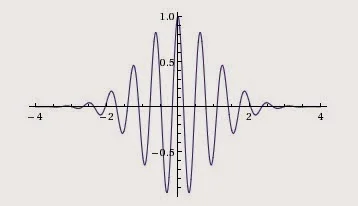
The integrand cos(10x)e−1/2x2
The factor e−(1/2)σ2 dampens these oscillations, and in the end the result is simple: It is as if the cosine function wasn't even there, and just replaces σ by z. But a Monte Carlo evaluation of this integral runs into the sign problem when z gets large and the oscillations become more and more violent. The numerical average converges very very slowly, which means that your computer has to run for a very long time to get a good estimate.
Now imagine calculating an expectation value where this problem occurs both in the numerator and the denominator. In that case, we have to deal with small but weakly converging averages both in the numerator and denominator, and the ratio converges even more slowly. For example, imagine calculating the "mean square"

The denominator of this ratio (for N=1) is the integral we looked at above. The numerator just has an extra σ2 in it. The N ("particle number") is there to just make things worse if you choose a large one, just as in nuclear physics larger nuclei are harder to calculate. I show you below the result of calculating this expectation value using the Monte Carlo approach (data with error bars), along with the analytical exact result (solid line), and as inset the average "sign" Φ of the calculation. The sign here is just the expectation value of


You see that for increasing z, the Monte Carlo average becomes very noisy, and the average sign disappears. For a z larger than three, this calculation is quite hopeless: sign 1, Monte Carlo 0.
I want to make one thing clear here: of course you would not use the Monte Carlo method to calculate this integral if you can do it "by hand" (as you can for the example I show here). I'm using this integral as a test case, because the exact result is easy to get. The gist is: if you can solve this integral computationally, maybe you can solve those integrals for which you don't know the answer analytically in the same manner. And then you solve the sign problem. So what other methods are there?
The solution I proposed was using the complex Langevin equation. Before moving to the complex version (and why), let's look at using the real Langevin equation to calculate averages. The idea here is the following. When you calculate an integral using the Monte Carlo approach, what you are really doing is summing over a set of points that are chosen such that you reject (probabilistically) those that are not close to the integrand--and you accept those that are close, again probabilistically, which creates a sequence of random samples that approximates the probability distribution that you want to integrate.
But there are other methods to create sequences that appear to be drawn from a given probability distribution. One is the Langevin equation which I'm going to explain. Another is the Fokker-Planck equation, which is related to the Langevin equation but that I'm not going to explain.
Here's the theory (not due to me, of course), on how you use the Langevin equation to calculate averages. Say you want to calculate the expectation value of a function O(σ). To do that, you need to average O(σ), which means you sum (and by that I mean integrate), this function over the probability that you find σ. The idea here is that σ is controlled by a physical process: σ does not change randomly, but according to some laws of physics. You want to know the average O, which depends on σ, given that σchanges according to some natural process.
If you think about it long enough, you realize that many many things in physics boil down to calculating averages just like that. Say, the pressure at room temperature given that the molecules are moving according to the known laws of physics. Right, almost everything in physics, then. So you see, being able to do this is important. Most of the time, Monte Carlo will serve you just fine. We are dealing with all the other cases here.
First, we need to make sure we capture the fact that the variable σ changes according to some physical law. When you are first exposed to classical mechanics, you learn that the time development of any variable is described by a Lagrangian function (and then you move on to the Hamiltonian so that you are prepared to deal with quantum mechanics, but we won't go there here). The integral of the Langrangian is called the "action" S, and that is the function that is used to quantify how likely any variable σ is given that it follows these laws. For example, if you are particle following the laws of gravity, then I can write down for you the Lagrangian (and hence the action) that makes sure the particles follow the law. It is L=−12mv2+mV(σ), where m is the mass, and v is the velocity of the σ variable, v=dσ/dt, and V(σ) is the gravitational potential.

In computational physics, what you want is a process that creates this equilibrium distribution, because if you have it, then you can just sum over the variables so created and you have your integral. Monte Carlo is one method to create that distribution. We are looking for another.
It turns out that the Langevin equation
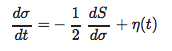
creates precisely such a process. Here, S is the action for the process, and η(t) is a noise term with zero mean and unit variance:

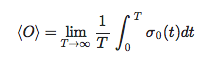
Note that t here is a "ficitious" time: we use it only to create a set of σs that are distributed according to the probability distribution P(σ) above. If we have this ficitious time series σ0 (the solution to the differential equation above), then we can just average the observable O(σ):
Let's try the "Langevin approach" to calculating averages on the example integral ⟨σ2⟩Nabove. The action we have to use is

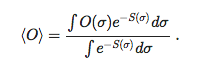
so that e−S gives exactly the integrand we are looking for. Remember, all expectation values are calculated as
With that action, the Langevin equation is

This update rule creates a sequence of σ that can be used to calculate the integral in question.
And the result is ..... a catastrophe!
The average does not converge, mainly because in the differential equation (1), I ignored a drift term that goes like ±iδ(cos(zσ)). That it's there is not entirely trivial, but if you sit with that equation a little while you'll realize that weird stuff will happen if the cosine is zero. That term throws the trajectory all over the place once in a while, giving rise to an average that simply will not converge.
In the end, this is the sign problem raising its ugly head again. You do one thing, you do another, and it comes back to haunt you. Is there no escape?
You've been reading patiently so far, so you must have suspected that there is an escape. There is indeed, and I'll show it to you now.
This simple integral that we are trying to calculate

we could really write it also as

because the latter integral really has no imaginary part. Because the integral is symmetric.
This is the part that you have to understand to appreciate this article. And as a consequence this blog post. If you did, skip the next part. It is only there for those people that are still scratching their head.
OK: here's what you learn in school: eiz=cos(z)+isin(z). This formula is so famous, it even has its own name. It is called Euler's formula. And cos(z) is a symmetric function (it remains the same if you change z→−z), while sin(z) is anti-symmetric (sin(−z)=−sin(z)). An integral from −∞ to ∞ will render any asymmetric function zero: only the symmetric parts remain. Therefore, ∫∞−∞eiz=∫∞−∞cos(z).
This is the one flash of brilliance in the entire paper: that you can replace a cos by a complex exponential if you are dealing with symmetric integrals. Because this changes everything for the Langevin equation (it doesn't do that much for the Monte Carlo approach). The rest was showing that this worked also for more complicated shell models of nuclei, rather than the trivial integral I showed you. Well, you also have to figure out how to replace oscillating functions that are not just a cosine, (that is, how to extend arbitrary negative actions into the complex plane) but in the end, it turns out that this can be done if necessary.
But let's first see how this changes the Langevin equation.
Let's first look at the case N=1. The action for the Langevin equation was

If you replace the cos, the action instead becomes
The fixed point of the differential equation (1), which was on the real line and therefore could hit the singularity $\delta(\cos(z\sigma))$, has now moved into the complex plane.
And in the complex plane there are no singularities! Because they are all on the real line! As a consequence, the averages based on the complex action should converge! The sign problem can be vanquished just by moving to the complex Langevin equation!
And that explains the title of the paper. Sort of. In the figure below, I show you how the complex Langevin equation fares in calculating that integral that, scrolling up all the way, gave rise to such bad error bars when using the Monte Carlo approach. And the triangles in that plot show the result of using a real Langevin equation. That's the catastrophe I mentioned: not only is the result wrong. It doesn't even have large error bars, so it is wrong with conviction!
The squares (and the solid line) come from using the extended (complex) action in the Langevin equation. It reproduces the exact result precisely.

Average calculated with the real Langevin equation (triangles) and the complex Langevin equation (squares), as a function of the variable z. The inset shows the "sign" of the integral, which still vanishes at large z even as the complex Langevin equation remains accurate.
The rest of the paper is somewhat anti-climactic. First I show that the same trick works in a quantum-mechanical toy model of rotating nuclei (as opposed to the trivial example integral). I offer the plot below from the paper as proof:

But if you want to convince the nuclear physicists, you have to do a little bit more than solve a quantum mechanical toy model. Short of solving the entire beast of the nuclear shell model, I decided to tackle something in between: the Lipkin model (sometimes called the Lipkin-Meshkov-Glick model), which is a schematic nuclear shell model that is able to describe collective effects in nuclei. And the advantage is that exact analytic solutions to the model exist, which I can use to compare my numerical estimates to.
The math for this model is far more complicated and I spare you the exposition for the sake of sanity here. (Mine, not yours). A lot of path integrals to calculate. The only thing I want to say here is that in this more realistic model, the complex plane is not entirely free of singularities: there are in fact an infinity of them. But they naturally lie in the complex plane, so a random trajectory will avoid them almost all of the time, whereas you are guaranteed to run into them if they are on the real line and the dynamics return you to the real line without fail. That is, in a nutshell, the discovery of this paper.
So, this is obviously not a well-known contribution. This is a bit of a bummer, because the sign problem still very much exists, in particular in lattice gauge theory calculations of matter at finite chemical potential (meaning, at finite density). Indeed, a paper came outjust recently (see the arXiv link in case you ended up behind a paywall) where the authors try to circumvent the sign problem in lattice QCD at finite density by doing the calculations explicitly at high temperature using the old trick of doubling your degrees of freedom. Incidentally, this is the same trick that gives you black holes at Hawking temperature, because the event horizon naturally doubles degrees of freedom. I used this trick a lot when calculating Feynamn diagrams in QCD at finite temperature. But that's a fairly well-known paper, so I can't discuss it here.
Well, maybe some brave soul one day rediscovers this work, and writes a "big code" that solves the problem once and for all using this trick. I think the biggest reason why this paper never got any attention is that I don't write big code. I couldn't apply this to a real-world problem, because to do that you need mad software engineering skills. And I don't have those, as anybody who knows me will be happy to tell you.
So there this work lingers. Undiscovered. Lonely. Unappreciated. Like sooo many other papers by sooo many other researchers over time. If only there was a way that old papers like that could get a second chance! If only :-)
[1] H. Gausterer, Complex Langevin: A numerical Method? Nuclear Physics A 642 (1998) 239c-250c.
[2] C. Adami and S.E. Koonin, Complex Langevin equation and the many-fermion problem. Physical Review C 63 (2001) 034319.
